Deep Learning-Assisted Quantitative Measurement of Thoracolumbar Fracture Features on Lateral Radiographs
Article information

Abstract
Objective
This study aimed to develop and validate a deep learning (DL) algorithm for the quantitative measurement of thoracolumbar (TL) fracture features, and to evaluate its efficacy across varying levels of clinical expertise.
Methods
Using the pretrained Mask Region-Based Convolutional Neural Networks model, originally developed for vertebral body segmentation and fracture detection, we fine-tuned the model and added a new module for measuring fracture metrics—compression rate (CR), Cobb angle (CA), Gardner angle (GA), and sagittal index (SI)—from lumbar spine lateral radiographs. These metrics were derived from six-point labeling by 3 radiologists, forming the ground truth (GT). Training utilized 1,000 nonfractured and 318 fractured radiographs, while validations employed 213 internal and 200 external fractured radiographs. The accuracy of the DL algorithm in quantifying fracture features was evaluated against GT using the intraclass correlation coefficient. Additionally, 4 readers with varying expertise levels, including trainees and an attending spine surgeon, performed measurements with and without DL assistance, and their results were compared to GT and the DL model.
Results
The DL algorithm demonstrated good to excellent agreement with GT for CR, CA, GA, and SI in both internal (0.860, 0.944, 0.932, and 0.779, respectively) and external (0.836, 0.940, 0.916, and 0.815, respectively) validations. DL-assisted measurements significantly improved most measurement values, particularly for trainees.
Conclusion
The DL algorithm was validated as an accurate tool for quantifying TL fracture features using radiographs. DL-assisted measurement is expected to expedite the diagnostic process and enhance reliability, particularly benefiting less experienced clinicians.
INTRODUCTION
Thoracolumbar (TL) fractures often manifest with vertebral deformities as the fractures progress, resulting in decreased vertebral body (VB) height and the development of spinal kyphosis [1-3]. Quantitative measurements of vertebral height, compression rate (CR), and kyphotic angles, primarily conducted using plain radiographs, are essential not only for clinical evaluation but also for surgical reimbursement criteria. Many insurance providers base their coverage decisions on criteria such as the presence of unstable spinal fractures, such as burst fractures with a kyphotic angle greater than 30°, a compression ratio above 40%, or spinal canal invasion exceeding 50%. Despite the simplicity of these measurements, they are often repetitive and time-consuming due to the use of various measurement methods and subject to significant interobserver variance [4-6].
Deep learning (DL) algorithms, particularly employing convolutional neural networks (CNNs) as a computer vision, have gained significant interests in the various medical fields due to their remarkable potential for improving diagnostic accuracy and workflow efficiency [7-12]. In the spine researches, many studies have been conducted on detecting vertebral fractures [13,14], and segmenting the VB with sagittal parameter measurement [15-18]. These approaches have demonstrated excellent efficacy, leading to the introduction of several commercially available software solutions for preoperative planning in spinal deformity surgery [19,20].
However, there is still a lack of DL research focused on the quantitative measurement of TL fracture features, which requires precise segmentation of fractured VBs. Current DL models for semantic segmentation, designed for binary classification, perform well on intact VBs, but struggle with fractured VBs, which are often deformed and overlapped with adjacent VBs [14,21]. To address this challenge, it is crucial to employ an appropriate DL algorithm for instance segmentation. Hence, this study aimed to develop and validate a relevant DL algorithm specifically for the quantitative measurement of TL fracture features using plain radiographs.
MATERIALS AND METHODS
This retrospective study was approved by both the Institutional Review Board (No. 2022-08-008) and the Institutional Big Data Research Ethics Committee. Any patient information was anonymized prior to image acquisition, and the requirement for informed consent was waived due to the retrospective nature of the study.
1. Data Collection and Study Population
Two patient cohorts were included in this study. The nonfracture group comprised patients who underwent lumbar spine radiography at our hospital's emergency medicine, orthopedic surgery, and neurosurgery departments between November 2021 and January 2022. The fracture group consisted of patients diagnosed with TL fractures who underwent lumbar spine radiography from January 2015 to January 2022. The exclusion criteria for the nonfracture group included patients with severely impaired image quality, inappropriate field of view (either too wide or too small), presence of spinal surgical instrumentation, limitations in imaging evaluation (e.g., due to vertebroplasty or other surgical factors, presence of artifacts or contrast agents obstructing evaluation), pathological fractures (e.g., due to tumors, infections, inflammation), severe spinal deformities (e.g., severe scoliosis or kyphosis), and congenital spinal anomalies. In the fracture group, we additionally excluded patients with 3 or more consecutive vertebral fractures, or fractures outside the VB (e.g., spinous process or transverse process).
In total, 1,531 cases (1,000 nonfracture cases and 531 fracture cases) were collected. For training, 1,000 nonfracture cases and 318 fracture cases were used, and for internal validation, 213 fractured cases were used. Additionally, for external validation, we collected 200 fracture cases from another tertiary hospital using the same selection criteria. There was an imbalance in the training dataset between nonfractured cases and fractured cases, which reflects the actual prevalence of TL fracture, as fractures are relatively less common compared to nonfractured cases. However, with a large number of nonfractured cases, the model can be further fine-tuned for the 6-point labeling accuracy and segmentation performance.
2. Image Data Acquisition and 6-Point Labeling
The lateral view of lumbar spine plain radiographs, covering T10 to S5, were obtained in Digital Imaging and Communications in Medicine (DICOM) file format. After image acquisition, no special preprocessing was applied to the radiographs before labeling. The original DICOM images were directly transferred to the labeling platform, which allows for basic image adjustments such as brightness, contrast, saturation, and hue, along with a magnification feature. Three musculoskeletal radiologists, each with more than a decade of clinical experience, were assigned the task of independently labeling one-third of the dataset. Following their individual labeling works, a final review was conducted by one radiologist to ensure accuracy and consistency. In cases where significant disagreements arose during the final review, they were thoroughly discussed to reach a consensus and finalized the decisions. The results of the final decision were considered to be the ground truth (GT). We adopted a 6-point labeling method for the quantitative measurement of TL fracture features [22,23]. For nonfractured vertebrae, 6 points were marked on each VB (Fig. 1): 4 at the corners and 2 additional points at the midportion of the superior and inferior endplates. These 6 points form 3 pairs—anterior, middle, and posterior. For the fractured vertebrae, the anterior and posterior points were marked in the same manner, while the middle points were placed at the smallest height location. Lines were drawn between each pair, perpendicular to the endplates, enabling accurate assessment of the anterior, middle, and posterior heights of the VB. The heights at the anterior, middle, and posterior VB were measured as the distance between the respective paired points. For fractured VBs, the smallest of these 3 heights was taken as the representative height. In cases where one of the adjacent VBs could not be measured, the height of the counterpart was taken as the average.
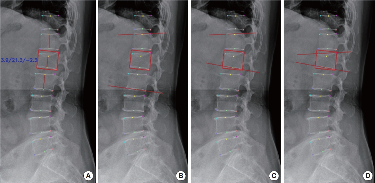
Measurement of the compression rate and kyphotic angles based on 6-point labeling. Automated detection of a fractured vertebral body (VB) with a bounding box is demonstrated. Lines connecting the superior and inferior corner dots define the superior and inferior endplate lines, respectively. (A) Compression rate is calculated by the ratio of the reduced height of the fractured VB to the average height of the adjacent VBs (1–[height of fractured VB/mean height of adjacent VBs]). The blue numbers display the compression rates (%) of the anterior, middle, and posterior parts of the VB. The smallest value among these is selected as the representative compression rate. (B) Cobb angle is measured between the superior endplate of the upper adjacent VB and the inferior endplate of the lower adjacent VB. (C) Gardner angle is measured between the superior endplate of the upper adjacent VB and the inferior endplate of the fractured VB. (D) Sagittal index is calculated as the angle between the superior and inferior endplates of the fractured VB.
Various ambiguous situations of the 6-point labeling and its corresponding rules are illustrated in Supplementary Fig. 1. Recognizing the variability in fracture types, particularly the more intricate C and D types, we made rules to label in various situations, to mitigate errors and improve inter- and intraobserver reliability in our measurements. This was critical to ensure reproducibility and consistency, especially since fractures can present as combinations (e.g., A+C or B+D). Supplementary Fig. 2 showed the rules of measuring fracture features in presence of 2 consecutive VB fractures. When 2 VBs are involved, the CR is calculated using the height of one adjacent unfractured VB. The Cobb angle (CA), Gardner angle (GA), and sagittal index (SI) are measured in the same manner as with other types of fractures.
3. Quantitative Metrics of TL Fracture Features
Various metrics for TL fracture features have been introduced and studied [5,24-26]. Among them, we evaluated the CR, CA, GA, and SI. The CR is calculated by comparing the height of the fractured VB with the mean height of the adjacent upper and lower VBs. The formula was: CR= (1–height of the fractured VB/mean height of the upper and lower adjacent VBs)× 100%. The CA was determined as the angle between the lines of the upper endplate of the upper adjacent VB and the lower endplate of the lower adjacent VB. The GA measures the angle between the upper endplate of the upper adjacent VB and the lower endplate of the fractured VB. The SI was calculated as the angle between the upper and lower endplate lines of the fractured VB (Fig. 1).
4. Development of a DL Algorithm
1) DEEP:SPINE
In our previous study, the automatic spinal disease analysis software, DEEP:SPINE (DEEPNOID Inc., Seoul, Korea) was developed; this software was originally designed for the detection and segmentation of all visible VBs, including fractured VBs, from spine radiography [14]. DEEP:SPINE utilized Detectron2 library [27], a Mask Region-based Convolutional Neural Network (Mask R-CNN) model designed specifically for object instance segmentation, via the transfer learning method [16,28].
During the development of DEEP:SPINE, we compared U-Net-based and Mask R-CNN based models (Supplementary Fig. 3). The Dice similarity coefficient values with standard deviations for U-Net and Mask R-CNN were 0.895 ± 0.052 and 0.939 ± 0.029, respectively, demonstrating that Mask R-CNN consistently outperformed U-Net in VB segmentation. This can be attributed to the different segmentation approaches used: U-Net, which performs semantic segmentation, faces challenges in accurately delineating overlapping or deformed VBs. In contrast, Mask R-CNN, which specializes in instance segmentation, detects regions of interest (ROI) prior to segmentation, thereby offering improved precision. For these reasons, we selected the Mask R-CNN model for the DEEP:SPINE software due to its suitability for our specific segmentation tasks.
In this study, we further fine-tuned the pretrained DEEP: SPINE model to improve its suitability for fractured VB segmentation [27]. Additionally, we developed new modules to quantitatively measure fracture features, thereby establishing a novel 2-step DL algorithm that integrates the fine-tuned DEEP:SPINE framework with the newly developed modules. The process of deriving quantitative TL fracture features consisted of 3 stages, as outlined below (Fig. 2).
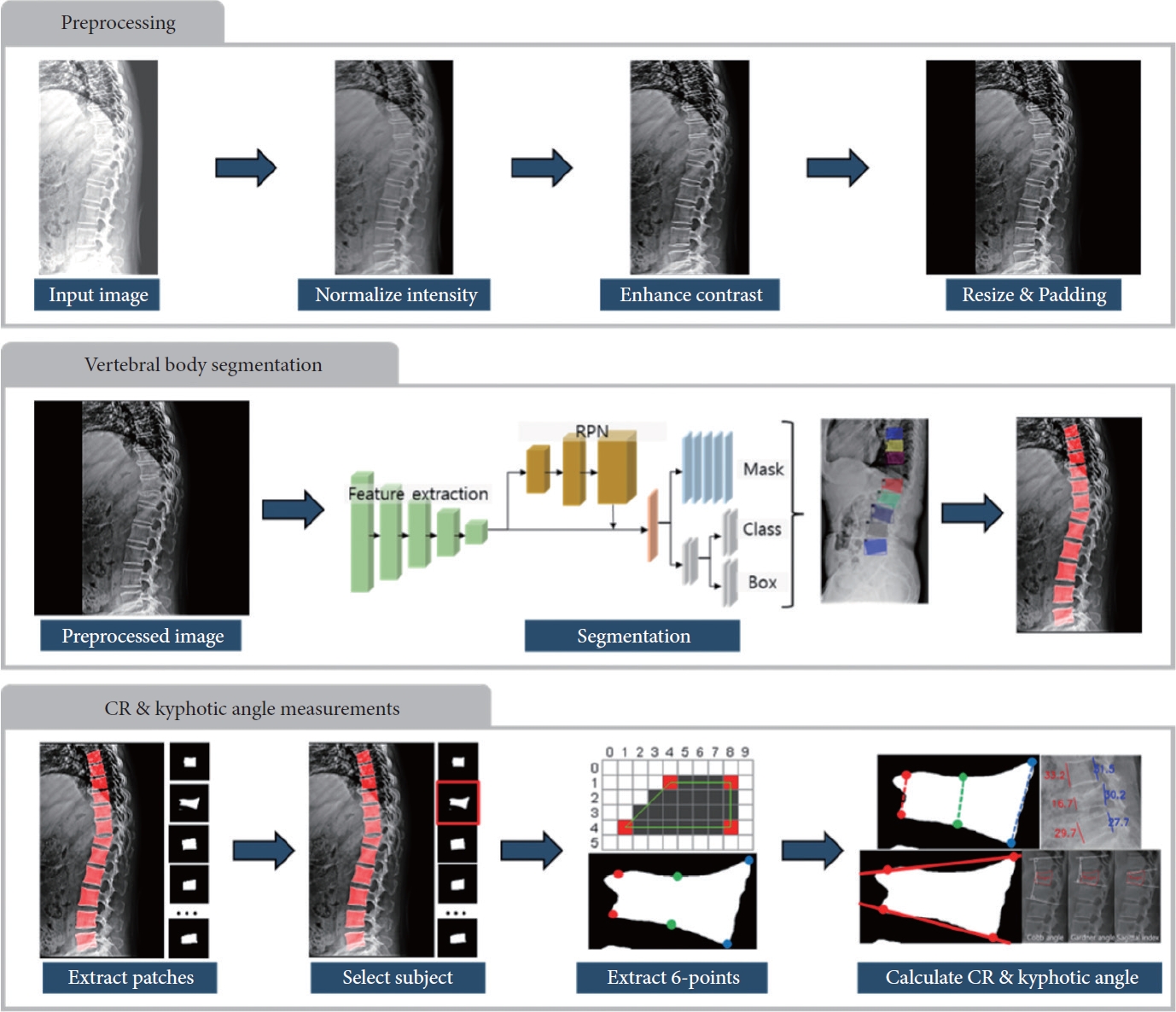
Sequential pipeline for deep learning-based quantitative analysis of TL fracture features. The diagram outlines the stepby- step workflow of the developed deep learning-based algorithm for analyzing quantitative features related to TL fractures. The pipeline includes data preprocessing, Mask R-CNN based vertebral body segmentation, and subsequent stages focused on measuring CR and kyphotic angles. RPN, Region Proposal Network; TL, thoracolumbar; Mask R-CNN, Mask Region-Based Convolutional Neural Networks; CR, compression rate.
(1) Stage 1: Preprocessing
The initial stage involved the preprocessing of L-spine radiography images to enhance their quality and prepare them for subsequent analysis. This stage encompassed the following key steps.
- Normalization: Radiography images underwent a normalization process to ensure consistent intensity levels across all images.
- Contrast enhancement: We applied the Contrast Limited Adaptive Histogram Equalization (CLAHE) algorithm to enhance image quality and improve the visibility of critical features. CLAHE is one of the most popular image processing techniques to enhance the quality of radiographs, especially for spine or bone segmentation [29]. Albeit high computational costs are a concern, the enhanced accuracy due to the clarity of the resulting image justifies these costs. A clip limit of 100 and a tile grid size of (8,8) were set as the parameters, which were suggested by Pan et al. [30] to optimize the performance.
- Resizing: Images were resized to a standardized dimension of 512 by 512 pixels, while maintaining the original image’s aspect ratio through zero-padding.
(2) Stage 2: VB segmentation
In the second stage of our methodology, automated VB segmentation was performed on the preprocessed radiography images using Mask R-CNN. This advanced CNN architecture comprises 3 crucial components: a backbone network responsible for feature extraction, a Region Proposal Network generating candidate object region proposals, and a mask head that handles object classification, bounding box regression, and instance mask prediction. To train this model, mask images representing hexagonal regions corresponding to the 6-point labels assigned to VBs were utilized. The training process involved configuring the model with the following specific parameters: an Adam optimizer initialized with an initial learning rate of 0.001, further optimized by the Warmup-Cosine learning rate scheduler. We employed a configuration with a maximum of 128 ROIs per image, conducted training for 100 epochs, and used a batch size of 32 images. Therefore, considering the total dataset size (1,318), batch size (32), and number of epochs (100), the training phase involved a total of 4,800 iterations. Furthermore, we added random augmentations of random horizontal flips, rotation from -10° to 10°, random brightness adjustment from range of 0.5 to 2, and random contrast from range 0.9 to 1.1. During the training phase, a multitask loss function was employed, encompassing object classification loss (log loss), bounding box regression loss (smooth L1 loss), and segmentation loss (binary cross-entropy loss). The equation for total loss and all the individual losses are as below:
where L represents loss function.
where C represents number of classes, yc represents the binary indicator (0 or 1) of whether class label c is the correct classification for the prediction, and pc is the predicted probability of the observation being of class c.
where xn represents the predicted value, yn represents the GT value, and N represents the total number of elements in the output. β is the arbitrary threshold parameter that determines the point at which the loss transitions from a quadratic to linear function. We set 1.0 as the value for β which is the default and most generally used value for the term.
where m is the predicted probability of the positive class, and n is the binary indicator (0 or 1) of whether the GT is the positive class.
Classification loss (LClassification) penalizes incorrect class predictions, bounding box loss (LBbox) penalizes by the incorrectness of the box coordinates, and mask loss (LMask) penalizes the inaccurate prediction in the pixel-level segmentation object. This comprehensive loss function guided the model in achieving accurate object classification, precise bounding box refinement, and the generation of high-fidelity instance masks. For model training, the Detectron2 framework (https://github.com/facebookresearch/detectron2) [27], built upon the PyTorch framework, was utilized. Moreover, we used the publicly available pretrained weights provided in the Detectron2 package, which have been trained on the popular COCO instance segmentation dataset. The training process was executed on a dedicated single GPU server equipped with 512GB of RAM memory, an Intel Xeon E5-2640 v4 CPU, and 8ea TITAN XP GPUs by NVIDIA. These hardware and software resources collectively provided the computational capacity required for training our Mask R-CNN model effectively.
(3) Stage 3: Quantitative measurement of TL fracture features
In the final stage, patches corresponding to each segmented VB were extracted from the predicted mask images generated by the segmentation model. Within each selected subject VB, the labeling data of 6 points were extracted, forming the basis for measuring CR, CA, GA, and SI. This comprehensive approach constituted the fundamental process of our measurement methodology. This automated process utilizes image preprocessing, DL techniques, and statistical algorithms for accurate measurements.
5. Evaluation of the DL Algorithm Performance
1) Agreement of the DL algorithm with the GT
Since the measurements do not have a specific correct answer, achieving consistency with or the closest value to the GT indicates high performance. Four key metrics—CR, CA, GA, and SI—were calculated for both internal and external validations, followed by their agreement between the GT and the DL algorithm (Fig. 3).

Comparison of compression rate with 6-point labeling on thoracolumbar spinal radiographs by ground truth (GT) and a deep learning (DL) algorithm. Every visible vertebral body (VB) is marked with 6 points indicating the anterior, middle, and posterior columns. (A) Simple compression fracture. GT and DL labels nearly identical. (B) Failure of DL to place the middle upper point at the lowest site of the VB. (C) Incorrect placement of the middle pair by DL, suggesting difficulty in interpreting the 3-dimensional structure of a fractured VB from a nontrue lateral view 2-dimensional radiograph. The blue numbers indicate the compression rates (%) for the anterior, middle, and posterior parts of the VB.
2) Performance of different levels of readers without DL algorithm assistance
Four readers with varying clinical experience from our institution participated in this evaluation: a second-year neurosurgery trainee, second- and fourth-year radiology trainees, and an attending spine neurosurgeon with 7 years of experience after neurosurgery board certification. Each reader performed 6-point labeling on both the internal and the external validation datasets. Four metrics were derived from these labels. Agreement with the GT for each metric was obtained for each reader.
3) Performance of readers with DL algorithm assistance
A month after the initial labeling session, the 4 readers revisited the labeling task, this time with the assistance of the DL algorithm, on the same internal and external datasets. In this second round, the readers adjusted 6 preidentified points suggested by the DL algorithm, refining their positions as necessary.
6. Statistical Analysis
The demographic characteristics of both the nonfracture and fracture groups were analyzed using descriptive statistics. Since this task involves quantitative measurements without a definitive correct answer, we considered the labeling results of the experienced radiologist as the reference (meaning GT), and compared the results of the DL algorithm with the GT. The agreement between the GT and the DL algorithm was analyzed using the intraclass correlation coefficient (ICC) values: less than 0.5, between 0.5 and 0.75, between 0.75 and 0.9, and greater than 0.90 are indicated poor, moderate, good, and excellent reliability, respectively.31 Paired t-tests were used to compare values between measurements without and with DL assistance for each reader, to investigate the impact of the DL assistance. All the statistical analyses were carried out using R software (ver. 4.0.5, R Foundation for Statistical Computing, Vienna, Austria).
RESULTS
1. Demographics and Baseline Characteristics
Table 1 summarizes the baseline characteristics and fracture distributions of a total of 1,731 patients from the internal and external datasets. Within the internal dataset, the nonfracture group consisted of 522 males (52.2%) and 478 females (47.8%) with a mean age of 49.4 years (range, 19–89 years; standard deviation [SD], 16.2), whereas the fracture group included 152 males (30.5%) and 369 females (69.5%) with a mean age of 68.3 years (range, 19–101 years; SD, 14.5). The external dataset included 200 fracture cases, for which the gender ratio was 111 males (55.5%) to 89 females (44.5%). There were statistically significant demographic differences between the internal and external validation datasets, in terms of mean age and gender distribution (both with p< 0.01). The internal set, reflecting the training dataset, included a higher proportion of older females, while the external set included a greater number of younger males, with a lower incidence of degenerative and osteoporotic changes. Across all datasets, the most frequent sites of fractures were observed at L1, T12, and L2 levels, accounting for approximately 70% of cases in each test set.

Patient demographics and baseline characteristics
2. Evaluation of the DL Algorithm Performance
1) Agreement between the GT and the DL algorithm
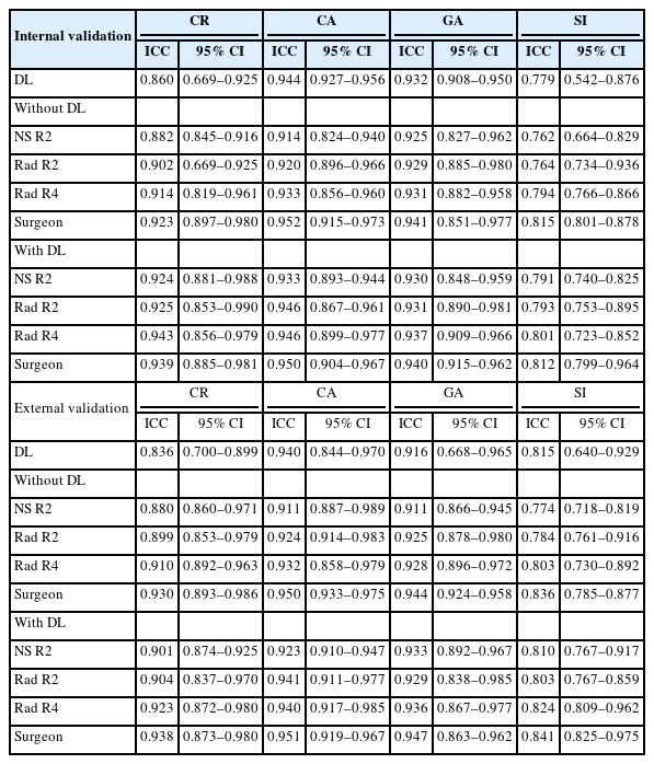
The DL algorithm demonstrated good to excellent agreement with the GT. In the internal validation, ICC values for CR, CA, GA, and SI were 0.841, 0.944, 0.932, and 0.776, respectively. In the external validation, the 4 measurement values were 0.836, 0.940, 0.916, and 0.815, indicating consistent and reliable results (Table 2, Fig. 4).
Performance of readers with or without DL assistance

Intraclass correlation coefficient plots between the deep learning algorithm and ground truth. ICC, intraclass correlation coefficient; CR, compression rate; CA, Cobb angle; GA, Gardner angle; SI, sagittal index; GT, ground truth; DL, deep learning.
2) Agreement between the GT and readers without DL algorithm assistance
The readers exhibited good to excellent agreement with the GT across all the metrics. Among the readers, the attending spine surgeon, fourth-year radiology trainee, second-year radiology trainee, and second-year neurosurgery trainee had the highest to lowest ICC values for all the measurements (Table 2). On average, the ICC values of the readers for CR were superior, while for CA and GA, they were comparable. For the SI, the values were slightly lower than those achieved by the DL algorithm in both validation sets (Fig. 5).
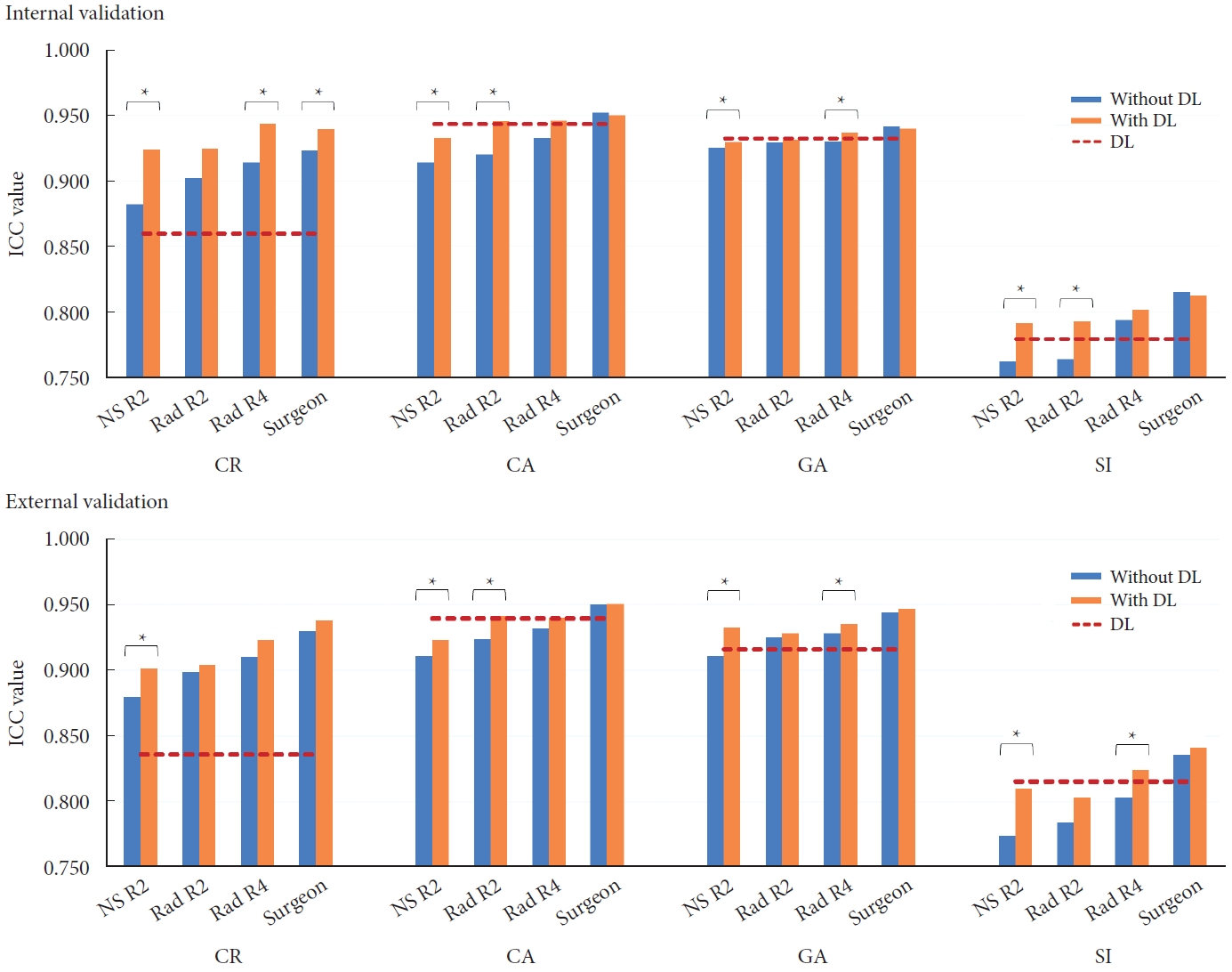
Comparison of performance among the 4 readers for CR, CA, GA, and SI, without and with the DL assistance. An asterisk denotes a significant difference with p<0.05 by paired t-test. NS R2, neurosurgery second-year resident; Rad R2, radiology second-year resident; Rad R4, radiology fourth-year resident; DL, deep learning; ICC, intraclass correlation coefficient; CR, compression rate; CA, Cobb angle; GA, Gardner angle; SI, sagittal index; GT, ground truth.
3) Agreement between the GT and readers with DL algorithm assistance
The ICC values indicated good to excellent agreement with the GT. Paired t-test analysis revealed statistically significant improvements in most metrics when utilizing the DL algorithm compared to without its assistance (Fig. 5). Notably, the trainees showed more substantial improvements compared to the attending spine surgeon (Table 2).
DISCUSSION
The key findings of this study reveal that the DL algorithm, employing the Mask R-CNN model, successfully measured the various quantitative metrics of TL fracture. The results exhibited good to excellent agreement with the assessments of an experienced musculoskeletal radiologist. Furthermore, DL-assisted measurements showed an improvement for radiology and neurosurgery trainees compared to their assessments without DL assistance.
CNN models, key algorithms in computer vision, have been increasingly applied in spinal image analysis. Li et al. [13] utilized DL techniques to detect osteoporotic lumbar vertebral fractures in spinal radiographs. Similarly, Galbusera et al. [17] developed a fully automated method for measuring spinal parameters using a CNN model. Cho et al. [15] also demonstrated the effective automated measurement of lumbar lordosis through VB segmentation using the U-Net model with radiography images. The U-Net, a widely used CNN architecture in medical imaging analysis, is designed for efficient binary semantic segmentation with small biomedical image datasets [32]. However, the U-Net encounters limitations in tasks requiring the detection and instance segmentation of fractured and normal adjacent vertebrae, as binary segmentation may incorrectly classify overlapping vertebrae as a single entity, particularly in radiographs where such overlap is common. To address this issue, our study employed Mask R-CNN, which distinguishes individual objects within the same class [28].
R-CNN, was originally developed for object detection [33]. This evolved into Fast R-CNN [34] and then Faster R-CNN [35,36], and finally Mask R-CNN was introduced in 2017 [28]. Mask R-CNN represents a significant advancement in the realm of computer vision, specifically designed for object instance segmentation. Its distinctive feature lies in its capability for instance segmentation, enabling the identification and differentiation of individual instances of objects within an image. This is achieved through the simultaneous prediction of bounding boxes, class labels, and pixel-wise segmentation masks. Mask R-CNN has been widely utilized across various domains including medical image analysis. In spinal image analysis research, Kim et al. [16] reported the successful use of Mask R-CNN for measurement of sagittal radiographic parameters with automatic vertebral segmentation for nonfractured vertebrae without deformity. Additionally, Kónya et al. [21] compared segmentation performance of various semantic and instance segmentation algorithms, including Mask R-CNN model, demonstrating its effectiveness in segmenting spine radiography images, even with implants such as screws and cement. However, this study lacked validation to assess its clinical effectiveness. Our study emphasizes the need for precise detection of the vertebral contours, particularly the endplates, to accurately define the boundaries of the intervertebral spaces. Moreover, we applied transfer learning from a pretrained Mask R-CNN model, which had been trained for VB segmentation tasks on diverse range of datasets, encompassing spinal radiographs of both nonfractured and fractured patients. This pretraining phase equipped the model with a comprehensive understanding of VB features, enabling it to generalize seamlessly to our target segmentation task. This transfer learning strategy also offers an advantage in improvement of accuracy in segmenting VB even with relatively small datasets, particularly in scenarios where labeled data is limited.
While the 6-point placement has been a well-established method for semiquantitative evaluation of VB fractures [22,23], our study stands out as the first to apply the 6-point labeling method to automated measurements through the DL algorithm. Previous research has often employed a 4-point labeling technique, involving the marking the 4 corners of the VB, to measure various coronal angles [18,37,38] and sagittal parameters [15,16,18]. However, the limitations of the 4-point labeling method become apparent in accurately measuring CR, as the lowest height of a fractured VB is often located at the midpoint. Kim et al. [14] employed an eight-point labeling method and successfully detected and segmented of fractured lumbar vertebrae using radiographs; however, they did not extend their model for quantitative measurement of TL fracture features. In contrast, our study applied the six-point labeling method and has successfully developed a DL model that accurately measures both CR and various kyphotic angles.
Additionally, our findings revealed that clinicians with different experience levels improved their diagnostic performance by using the DL assistance, demonstrating its practical clinical applicability through a comprehensive evaluation. To date, this is the first study regarding automated measurement of TL fracture features using a DL algorithm. Our results showed several interesting findings. Firstly, the DL algorithm was inferior to the GT and all readers for the measuring CR. Despite training with GT annotation results for labeling middle pair dots, the DL algorithm still showed discrepancies compared to the GT. This limitation highlights a critical area where the algorithm falls short, as it struggles to accurately infer the actual three-dimensional structure from 2-dimensional radiographs—a task in which human doctors excel. Conversely, regarding the various kyphotic angle measurements, the performance of the DL algorithm mostly surpassed that of the readers. This could be due to the relative straightforwardness of labeling anterior and posterior pairs for calculating kyphotic angles, where the DL algorithm was more precise and consistent. Secondly, the accuracy of the measurements performed by different readers mostly tended to be in the order of the attending spine surgeon, the DL algorithm, the fourth-year radiology trainee, the second-year radiology trainee, and the second-year neurosurgery trainee. This ranking underscores the importance of individual clinical experience in the accuracy of measurement, positioning the accuracy of the DL algorithm between that of an attending surgeon and that of trainees. Lastly, while the accuracy of the trainees improved with the assistance of the DL algorithm, the attending surgeon did not exhibit increased accuracy in kyphotic angle measurements. These findings suggested that augmentation with DL may not always be beneficial, particularly for those who already outperform the DL algorithm.
Another aspect worth discussing is the demographic disparity between the internal and external datasets. Notably, there were significant demographic differences between the internal and external validation cohorts, particularly in terms of mean age and gender distribution. The external validation set included a greater proportion of younger males, resulting in a lower frequency of degenerative changes or osteoporotic vertebral fractures (OVFs), along with higher instances of high-energy fractures. Such fractures typically show clearer margins due to higher bone density in younger patients, which might have contributed to marginally better algorithm performance in the external validation. Nevertheless, our model was designed to be applicable to various types of TL fractures and was not limited to OVFs. This effective performance on the external dataset demonstrates the robustness and generalizability of our model.
This study has several limitations. Firstly, the dataset was small and imbalanced, which was a result of the difficulty of collecting fracture data in a single-center study. However, by implementing transfer learning and increasing the number of nonfractured samples, we demonstrated robust model performance. Future studies with larger and more balanced datasets could further enhance the performance of the DL model. Secondly, the limited number of clinicians for the reader study, which was only 4, may not represent the diversity of clinical expertise. Subsequent studies could benefit from a more uniform group of readers, particularly from a single department and with consistent experience levels, to provide more controlled validation conditions and potentially greater reliability of the results. Thirdly, since fracture types and situations of VBs can significantly impact the accuracy of the DL model performance, subgroup analysis among them would be valuable. However, since there are many overlaps between each subgroup, it was difficult to classify them into definite categories and perform a subgroup analysis. Moreover, while there are definitive answers for the existence of fractures, concrete answer for TL fracture features is lacking. Thus, we relied solely on the experienced radiologist’s GT for comparison, and our evaluation was limited to using ICC values. Lastly, this study did not compare the time taken to perform measurements with and without DL assistance, an aspect that could provide insights into efficiency or cost-effectiveness.
CONCLUSION
We developed and validated a DL algorithm as an automated assisting tool for the quantitative measurement of TL fracture features. The reliability of the algorithm has been validated, and the results are comparable to those of various clinicians. Integrating this DL algorithm into the clinical workflow is anticipated to expedite the diagnostic process and enhance the reliability of diagnoses, offering substantial benefits, particularly to trainees in clinical practice.
Supplementary Material
Supplementary Figs. 1-3 can be found via https://doi.org/10.14245/ns.2347366.683.
(A) Six-point labeling in nonfractured vertebral body (VB) with true lateral view radiograph. (B) For fractured vertebrae, while the corner points remain unchanged, the middle pair points are placed at the site of the most pronounced height reduction, considered in a 3-dimensional (3D) context. (C) In instances where the lateral radiograph is not a true lateral view, and the superior and inferior endplates are misaligned, we inferred the 3D anatomy of the VB and labeled the middle points for the appropriate VB height. The green dots represent the most appropriate labeling methods, but red or blue dots can serve as alternative methods. (D) For VBs with significant osteophytes or protruding fracture fragments, the anterior and posterior pairs of points are marked, conserving the original, undisturbed shape of the VB.
Measurement methods for 2 consecutive vertebral body fractures. CR, compression rate; CA, Cobb Angle; GA, Gardner angle; SI, sagittal index; VH, vertebral height.
Comparison of the semantic segmentation model (U-Net) and the instance segmentation model (Mask R-CNN). (A) Original image of the lateral spine radiograph. (B) Ground truth (GT) segmentation by an experienced radiologist using 6-point labeling. (C) Semantic segmentation by U-Net, which failed to failed to segment overlapped T11 and T12 vertebral bodies (VBs), independently. The segmentation was too fit to osteophytes and deformed VBs. (D) Instance segmentation by Mask R-CNN, with bounding boxes and contours in various colors, closely aligned with the GT and outperforming U-Net.
Notes
Conflict of Interest
The authors have nothing to disclose.
Funding/Support
This study received no specific grant from any funding agency in the public, commercial, or not-for-profit sectors.
Author Contribution
Conceptualization: EKK; Formal Analysis: BK, HY; Investigation: WTY, EKK, YSY, JL, KYL, YSY, KDA; Methodology: WTY, EKK, BK, HY; Project Administration: EKK; Writing – Original Draft: WTY, EKK; Writing – Review & Editing: WTY, EKK, BK, HY.
Acknowledgements
This manuscript was presented in the 5th Biospine Korea Annual Meeting in 2nd December 2023. I would like to express our gratitude to researchers Jiyun Lee and DaHae Park (Hallym University Dongtan Sacred Heart Hospital) for their assistance in labeling imaging data. Additionally, we are thankful to Professor Il Choi, from the Department of Neurosurgery at Hallym University Dongtan Sacred Heart Hospital, for inspiring this research.