


INTRODUCTION
Virtual and augmented reality have enjoyed increased attention in spine surgery [1-3]. Preoperative planning, navigation for pedicle screw placement, and surgical training are among the most studied areas of application [1]. When navigating a 3-dimensional (3D) virtual reconstruction, identifying osseous structures on computed tomography (CT) is crucial. To automate the otherwise time-consuming process of labeling vertebrae on each individual slice, we propose a fully automated pipeline. Improved precision, decreased errors due to human fatigue, and increased consistency are suggested as benefits of incorporating automatic segmentation into clinical practice [4,5]. Also, virtual or augmented reality applications or radiomic analysis rely on target structure identification and segmentation [6]. Spine segmentation has been employed for disease diagnosis and preoperative treatment planning [7,8]. Augmented reality navigation has also been shown to improve the precision of screw insertion compared to free hand approaches [9]. Exact delineations of target structures is necessary for this. Convolutional neural networks are increasingly used for medical image segmentation [10].
U-Nets are frequently used for this task, and their efficacy has been sufficiently demonstrated [11-14]. Commonly, a region of interest needs to be manually defined first to further divide the image into anatomical regions, before segmentation can be performed [4]. By applying state-of-the-art object detection methods—trained on the task of creating bounding boxes around each individual vertebra—a greater level of automation and potentially enhanced segmentation precision could be achieved [15,16].
This 2-stage approach enables training convolutional neural networks on slices with higher—or even native—resolution, potentially increasing vertebral detection precision. This so-called patch-wise segmentation has a variety of benefits, from improved memory efficiency to addressing class imbalance of small structures [17]. Various strategies for defining field of views are applied in the VerSe 20 Challenge [18]. For example, Chen et al. [18] use a 3D U-Net for localization by initially generating random patches and then use these predictions to crop precisely. Payer et al. [19] generate heatmaps of the spine, identify the centroid of the vertebrae and crop a 3D patch around it. Yet, no attempt at using You-Only-Look-Once (YOLO) algorithms for patch-generation has been made. This allows for adaptive patch size around the precise edges of the vertebra. In summary, in this pilot study, we evaluate the feasibility of segmenting CTs of the cervical, thoracic, or lumbar spine using the proposed 2-stage machine learning approach with object detection followed by semantic segmentation.
MATERIALS AND METHODS
1. Data Collection and Preprocessing
We utilized 3 datasets: one for training and a subset of 2 others for external evaluation.
The dataset used for training is publicly available (VerSe 20 Challenge) and consists of 214 patients from a variety of centers and vendors (Siemens, GE, Philips, and Toshiba). The dataset had the following inclusion criteria: Minimum age of 18, 7 fully visualized vertebrae (without counting sacral od transitional vertebrae) and minimum pixel spacing of 1.5 mm (craniocaudal), 1 mm (anterior-posterior), 3 mm (left-right) [20]. Exclusion criteria were traumatic fractures and bony metastases [18,20-22]. The respective labels (26 different labels for the vertebrae from C1 to L5) were created through a semiautomated process: Initially, suggestions were made by an algorithm, which were subsequently refined by human experts [18,20,21]. Two medical students, specifically trained on the task, manually corrected the suggestion by the algorithm in a laborious process. This was performed in the original image space. The labels were subsequently validated by a neuroradiologist. Since the suggested segmentation mask was a 3D volume, we assume that all slice directions were considered in subsequent refinement process. These labels incorporated within the VerSe 20 dataset were used as ground truth for model training. For training purposes, this dataset consisting of 214 patients was split into 173 for training and validation during training (on a random 20% of the images) and a holdout dataset of 41 patients for internal validation.
Subsequently, to evaluate the out-of-sample performance of our fully trained method, we chose to test its performance on 2 other unrelated datasets: for the first external evaluation, we used a COVID-19 dataset (CT images in COVID-19) consisting of chest CTs captured at the initial point of care [23-25] that show the thoracic spine. Second, we evaluated our pipeline on 20 liver CTs, which span the lumbar and thoracic spinal regions and have also been part of a semantic segmentation challenge called Medical Segmentation Decathlon, of which we used 1 of the 10 subsets (MSD T10) [26,27]. The corresponding ground-truth labels were obtained from the CT1kSpine dataset [28], that created them in a semiautomated fashion from a nnU-Net that was updated every 100 cases. We opted for these 2 external validation datasets for the following reasons. First, they were suitable for our purposes since they were publicly available. Second, the manual segmentations came from the same dataset as the labels for training. Third, we wanted to evaluate the robustness of our approach on CTs that were not centered on the spine.
2. Preprocessing
We resampled the voxel size to isotropic 1.0 × 1.0 × 1.0 and padded the images to be uniform in size for all dimensions. Intensities were windowed with a center of 300 and a range of 2,000 and normalized with respect to their minimum and maximum.
3. Model Development
The training process is visually depicted in Fig. 1. First, a YOLO algorithm, Version 8 and size medium, (YOLOv8m) was trained to regions of interest [29,30]. Similar to cars detecting pedestrians [31], this learned to identify each vertebral body level and to create a bounding box for this. These regions were then cropped to the box size with a small margin of 5 pixels to ensure all corners of the vertebrae were on the smaller image. After cropping, these extracted regions were resized to 256× 256 and used as input for 2D-U-Net training [11]. As a convolutional network, it extracts feature maps in the contracting path. After a rectified linear unit activation function introduces nonlinearity, a max pooling operation takes the highest feature from each two-by-two square to half the dimensions. Subsequently, the expansion path uses transposed convolutions to reverse the reduction in dimension of the contracting path. Concatenation of feature maps on each symmetrical level helps restore spatial information. Finally, a sigmoid activation function assigns pixel-wise values to the segmentation mask. Due to this reduction and expansion in size, the architecture can be visualized in the shape of a “U,” hence the name of the model architecture. The following platforms were used: Python 3.9.0 [32], Keras 2.5.0 [33], SimpleITK [34], and nibabel [35]. The training was conducted on a Nvidia RTX 3090 graphical processing unit (GPU).
As a result of hyperparameter tuning, the best-performing model was trained for 14 epochs using early stopping. The final U-Net architecture consisted of 96 starting neurons, a depth of 3 with 4 blocks on each level. Binary cross-entropy was used as loss function, and a batch size of 80 yielded the best performance.
4. Evaluation
Precision (positive predictive value), recall (sensitivity), and mean average precision (mAP) with a Jaccard threshold of 0.5 (mAP50) were assessed as standard bounding-box evaluation metrics [36]. Furthermore, mAP50-95, which corresponds to mAP with 10 Jaccard score steps from 0.5–0.95 with steps of 0.05, was implemented. In those, a box reaching the respective predefined threshold is considered to be a true positive. To put this into perspective, one of the best values for a benchmark dataset called COCO are 0.79 for mAP50 and 0.66 for mAP50-95 [37].
U-Net performance was determined by comparing Dice score, Jaccard score and the 95th percentile of the Hausdorff distance of labels and predictions [38-41]. Dice and Jaccard score are measures of overlap ranging from zero—indicating no congruence—to one for a perfect match. While the Dice score is defined as twice the area of overlap divided by the sum of both areas, the Jaccard score describes the intersection divided by the union. Both metrics are ultimately a quotient of the correctly classified region and the ground-truth mask. The Hausdorff distance analyses the distance between 2 sets of points that are derived from the edges of the segmentations.
Evaluation was performed on the held-out VerSe 20 data, as well as the 2 external validation datasets. Mean and standard deviation as well as median and interquartile range are reported where appropriate.
RESULTS
1. Cohort
A total of 173 CT scans were used for training, 41 for internal validation, and 20 for each of the 2 external validation sets. Patient and radiological information, as reported by the respective datasets, is summarized in Table 1. The training dataset consisted of (mean± standard deviation [SD]), 523± 48 coronary, 600± 267 axial, and 537± 358 sagittal slices. The first external validation set with liver scans was comprised of 533± 71 coronary, 512± 96 axial, and 533± 71 sagittal slices and the second, chest CT dataset, entailed 400± 57 slices in all dimensions. The entire VerSe 20 dataset with 300 patients (86 from 2019 with lower resolution and 214 new cases) consists of 144 female patients (48%), with a (mean± SD) age of 56.2± 17.6. A total of 4,142 (100%) individual vertebrae were labeled, of which 581 (14%) were cervical, 2,255 (54%) thoracic and 1,306 (32%) lumbar vertebrae.
2. Object Detection: Identifying and Labeling Each Vertebral Level
A pretrained YOLOv8m with over 25 million parameters was trained on 40’446 images for 57 epochs using an early stopping function. Evaluation of the training, internal validation (holdout), and pool external validation performance resulted in a mAP50-95 of 0.64, 0.63, and 0.09 across all classes. Table 2 depicts detailed results per class for all the evaluated datasets. Precision and recall for different confidence levels are shown in Fig. 2. Inference time per slice for training, internal validation and pool external validation was 3.2 msec, 3.2 msec, and 5 msec, respectively.
3. Semantic Segmentation: Delineating Bony Structures
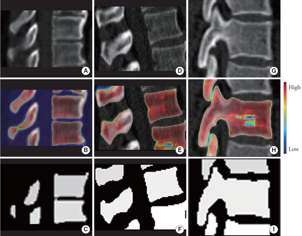
After object detection, single-vertebral-level cropped images were used to train and validate a semantic segmentation network: 94’184 cropped images were used for training. Training, internal validation (holdout), and pooled external validation showed a mean Dice of 0.75± 0.14, 0.76± 0.12, and 0.79± 0.1695, respectively. Detailed results are shown in Table 3. The distribution of the metrics is presented in Fig. 3. Exemplary results are depicted in Fig. 4. Following prediction, the cropped slices were reassembled into 3 dimensions. Inference time per slice for training, internal validation and pool external validation was 68 msec, 51 msec, and 44 msec.
DISCUSSION
We have developed and validated a pipeline for automated whole spine anatomical segmentation combining YOLO object detection and a 2D-U-Net for subsequent semantic segmentation. Generalizability was demonstrated by evaluating the performance on 2 different datasets for external validation. Our object detection method showed robust performance. By setting a low confidence threshold for detection, the risk of missing out on slices to segment is minimized. Segmentation was observed to yield robust results as well. At external validation, evaluation of our entire pipeline (semantic segmentation results) demonstrated robustness without signs of overfitting, as segmentation performance (incorporating the object detection method as a preprocessing step) was equal to training set performance.
Segmentation of medical imaging has become one of the major fields of clinical machine learning for many reasons within the last decade: Applications such as automated diagnostics and volumetric measurements, radiomics, and generation of virtual or augmented reality visualizations for demonstration, surgical training, and intraoperative navigation all necessitate robust methods for segmenting anatomical structures from native x-ray, CT or magnetic resonance imaging data [42-44]. However, the process of manually segmenting images—or manually correcting pre-segmented or thresholded images in the sense of semiautomated approaches—is highly time-consuming and would render broad adoption of the abovementioned applications into the clinical routine impossible [45].
Machine learning methods have thus markedly helped to cut down on time and effort needed for creating segmentations of medical images: For example, subarachnoid blood, intra-axial brain tumors, or pituitary adenomas can be readily segmented in a fully automated approach, in a time-efficient manner [46-48].
Normally, medical images are preprocessed and directly segmented by an algorithm, or specific regions of interest have to be manually delineated before segmentation, which is resource intensive and a potential source of errors. The spine is a large anatomical structure with clearly delineated segments (vertebral levels) and – at the bony level – regular interruptions (disc spaces), which would theoretically enable the use of object recognition algorithms to parcellate the spine into multiple smaller structures. Those extracted subregions can then be fed into algorithms with native or near-native resolution for a more precise and computationally efficient bony structure delineation. In addition, the obvious added benefit of object detection here is that vertebral levels are automatically recognized and labeled (for example, C7). From a generated segmentation, numerous parameters can be extracted. Hohn et al. [49] used a simpler thresholding approach combined with manual segmentation of subregions to determine bone quality. Maintaining high resolution data of the initial CT only helps generate more accurate estimations of bone mineral density. Siemionow et al. [50] assessed various parameters from segmenting spinal subregions. Those include vertebral body width, spinous process height, pedicle angulation and diameter at the isthmus. This provides the basis for automated operative planning, potentially assisting novice surgeons or reducing time needed for preoperative planning. These 2 examples not only illustrate the potential applications of automated spine segmentation, but also show the importance of high resolution patches without downsampling of image resolution.
We present a pilot study evaluating the feasibility and preliminary results of applying such a 2-stage automated segmentation pipeline, and generally shows that the concept is feasible and generalizes well to new images. Importantly, the external validation performance of the entire pipeline (semantic segmentation) was excellent—while the external validation performance of the object detection method itself seemed slightly less robust, which is partially inherent to the mAP metric. It is biased by model confidence, which tends to be lower during evaluation and, therefore, is more likely to fall below our predefined threshold. This trend can be seen in Fig. 2: External validation performance at a predetermined low confidence is inferior. Model confidence will be lower on new datasets, especially datasets that vary greatly from the training data, such as the liver and chest CTs used for external validation. Lower confidences do not necessarily equal worse bounding box generations, and the fact that final segmentation performance during external validation (building on the bounding boxes generated by our object detection algorithm) was still excellent is another indicator that our approach appears robust. Previous work with different approaches has yielded similar or even higher segmentation performance metrics [18]. This can mostly be attributed to 2 factors: First, we used rigorous 2-dimensional (2D) metrics since we performed our training on slices and not 3D volumes. On average, this will result in inferior performance (compared to e.g., 3D metrics), especially since we sometimes cropped segmentations made up only of a few pixels, and generally evaluated small volumes (spinal segments individually). One wrong pixel consequently has a bigger influence on measures of overlap compared to a full spinal imaging volume. This can be observed in Fig. 2 where the variability in metric performance becomes apparent. Secondly, our goal was to develop a clinically usable pipeline positioned at the optimal trade-off point between larger models’ demand for more computational resources while not compromising on performance [30]. Lastly, we aimed to develop one approach for the whole spine, whereas many other models are focused solely on a specific subregion of the spine.
As stated in the proceeding of the VerSe Challenge [18], a clinical spine CT scan is too large for GPU memory, and also for inference on clinical workstations with no designated GPU. Thus, either the resolution needs to be downsampled or the initial scan needs to be broken down into smaller pieces. As mentioned before, various techniques for this problem have been applied. We attempted to address this by a new, multistaged approach making use of the benefits of different models. The YOLO algorithms are largely used for real-time object detection, for example in autonomous driving where they are appreciated for their speed and precision [31]. U-Nets have been widely established in the field of biomedical image analysis [14]. Their main strength lies in precise segmentation, not detecting multiple objects on a large image. With 2D slices and cropping to a small portion of the initial image, we are able to drastically reduce the memory requirements of the input of the U-Net. For this pilot study, we also reduced image resolution for training, yet this is not a requirement for interference. With the implementation of a spatial pyramid pooling at the end of the YOLO architecture different input image scales can be efficiently handled [29,51]. For future inference, the CT could be used in native resolution for detection by the YOLO algorithm, and then cropped to the small patches. In then still native pixel scaling, the U-Net can be applied. In summary, we took the advantages of both models and combined them for optimal performance with reduced computational requirements.
With an ever increasing number of imaging studies carried out, automated supportive approaches such as ours can be of assistance in clinical practice [43], and accurate segmentation has the potential to impact clinical practice and efficiency. With inference times per slice of under 0.1 second for both models combined, they are well below the time manual segmentation requires. While pre- and postprocessing, using a non-GPU environment and processing all slices per series requires more time, human input time is minimized extensively. Also, our approach paves the way for accurate labeling and segmentation of more detailed anatomical structures such as foramina, articular processes, facets, laminae, and pedicles.
Even though segmentation performance was good at external validation, not the entire spectrum of real-world CT data, spine anatomy, and pathology are represented by the available datasets. Larger and more heterogeneous datasets would be advantageous to cover more variation. For two of the datasets that are fully anonymized, information on patients’ ages are not available, potentially limiting the generalizability of our results in different spine ages, for example in pediatric or geriatric patients. Also, training was partially confined in terms of model size and image resolution by computational constraints. Yet, smaller models usually have shorter inference times, which benefits potential applications to clinical routine on workstations without designated graphical processing units for machine learning. Equally, the image resolution had to be reduced for processing, resulting in pixelated masks if only a small region was cropped and then resized. This problem is inherent to our approach but could be reduced if training and predicting with higher pixel densities was less resource intensive. Finally, some regions of interest can be lost even with the high precision of our bounding box algorithm. Interpolating missing slices in postprocessing is feasible yet leads to a decrease in precision. Since we only trained on sagittal slices, mainly those are well segmented in 3 dimensions. Including slices from all dimensions and averaging the 3D predictions could reduce this effect in future work. Additionally, it could be hypothesized that more optimal, yet computationally demanding results could be achieved by using a 3D-U-Net. In order to minimize the input size, the mask generated by the YOLO algorithm could be applied to form a 3D volume, with the strategy described in our pilot study.
CONCLUSION
We propose a two-stage approach consisting of single vertebra labeling by an object detection algorithm followed by semantic segmentation. In our pilot study, including external validation, we demonstrate robust performance of our object detection network in identifying each vertebra individually, as well as for our segmentation model in exactly delineating the bony structures.